SCEG-HiC on paired scATAC-seq/scRNA-seq data of PBMC-CD4T
XuanLiang
Compiled: May 13, 2026
Source:vignettes/PBMC_multiomic_CD4T.Rmd
PBMC_multiomic_CD4T.RmdIn this vignette, we demonstrate the capability of SCEG-HiC to infer enhancer–gene links by applying it to paired scATAC-seq/RNA-seq data. Specifically, we use a publicly available 10x Genomics Multiome dataset from human PBMCs and select only CD4+ T cells for processing using the single-cell retention approach.
To begin, we require a Seurat object containing paired
scATAC-seq/scRNA-seq data. For this demonstration, we utilize publicly
available multi-omics dataset from human PBMCs, processed as described
in the SCEG-HiC
on paired scATAC-seq/RNA-seq data of PBMC (aggregation) The Seurat
object file, PBMC_multiomic.rds file is also available at
10.5281/zenodo.14849886.
Note: Due to the stochastic nature of
SCTransform, particularly in generating
scale.data, the UMAP embedding produced by re-running the
code may differ slightly from that in the provided
PBMC_multiomic.rds file.
The implementation of SCEG-HiC is seamlessly compatible with the standard workflow of the Seurat/Signac packages. The SCEG-HiC pipeline consists of the following two main steps:
Infer enhancer–gene links: Apply the SCEG-HiC model to the processed Seurat object, incorporating human bulk average Hi-C data as a chromatin conformation prior to enhance the inference of enhancer–gene links.
Visualize enhancer–gene links: Generate graphical outputs such as arc diagrams and coverage plots to visualize predicted enhancer–gene links.
Infer enhancer–gene links
Preprocess data
Here, we use the single-cell retention approach to handle paired scATAC-seq/RNA-seq data. The scATAC-seq counts are normalized using TF-IDF. We specifically select CD4+ T cells with paired scATAC-seq/RNA-seq data.
# Load processed multi-omics PBMC data
pbmc <- readRDS("PBMC_multiomic.rds")

# Prepare data for SCEG-HiC analysis
# Here, data is processed without aggregation, focusing on the CD4+ T cell type
SCEGdata <- process_data(pbmc, aggregate = FALSE, celltype = "CD4 T", rna_assay = "SCT", atacbinary = FALSE)
Calculate weight
Calculating weights with SCEG-HiC can be time-consuming, especially as the number of selected genes increases. To facilitate this process, SCEG-HiC provides downloadable average Hi-C datasets for both human and mouse (detail here). In this case, we select the human average Hi-C data as prior information to calculate enhancer-gene interaction weights.
As an example, we calculate Hi-C weights focusing on the CD4+ T cell marker gene GLB1.
# Alternatively, calculate Hi-C weights for the specific CD4+ T cell marker gene GLB1
weight <- calculateHiCWeights(SCEGdata, species = "Homo sapiens", genome = "hg38", focus_gene = "GLB1", averHicPath = "/mnt/netshare2/liangxuan/data/human_contact/AvgHiC")
## Processing chromosome chr3...## Found 1 TSS loci on chr3.## Calculating Hi-C weights for gene GLB1...## Finished calculating Hi-C weights for all genes.Run model
SCEG-HiC employs the wglasso method to infer enhancer-gene links by integrating processed single-cell multi-omics data and normalized bulk average Hi-C contact matrices. The bulk Hi-C matrix is normalized using rank score to improve accuracy. In this example, we run the model focusing on CD4+ T cell marker gene GLB1 to identify their putative enhancer links.
# Example: Run the model focused on Basal cell marker GLB1
results_SCEGHiC <- Run_SCEG_HiC(SCEGdata, weight, focus_gene = "GLB1")
## Total predicted genes: 1## Running model for gene: GLB1## [1] "The optimal penalty parameter (rho) selected by BIC is: 0.12"Visualize enhancer–gene links
Arc plot visualization of enhancer-gene links
Arc plot visualizes the predicted links between enhancers and target genes as arcs connecting genomic regions, highlighting spatial chromatin interactions inferred by SCEG-HiC.
Arc plot visualization of enhancer-gene links for GLB1.
# Download and prepare gene annotation data
# wget https://hgdownload2.soe.ucsc.edu/goldenPath/hg38/bigZips/genes/hg38.refGene.gtf.gz
temp <- "hg38.refGene.gtf.gz"
gene_anno <- rtracklayer::readGFF(temp)

# Rename some columns to match requirements
gene_anno$chromosome <- gene_anno$seqid
gene_anno$gene <- gene_anno$gene_id
gene_anno$transcript <- gene_anno$transcript_id
gene_anno$symbol <- gene_anno$gene_name

# Arc plot visualization of enhancer-gene links for GLB1
connections_Plot(results_SCEGHiC, species = "Homo sapiens", genome = "hg38", focus_gene = "GLB1", cutoff = 0.001, gene_anno = gene_anno)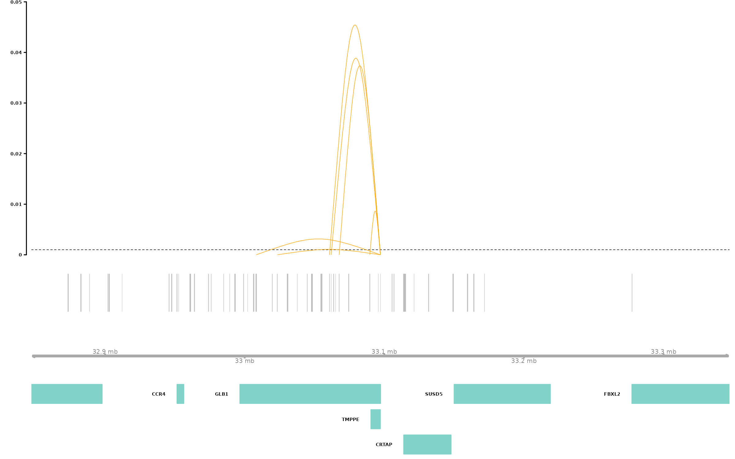
Session Info
## R version 4.4.2 (2024-10-31)
## Platform: x86_64-conda-linux-gnu
## Running under: Rocky Linux 9.6 (Blue Onyx)
##
## Matrix products: default
## BLAS/LAPACK: /home/liangxuan/conda/envs/test/lib/libopenblasp-r0.3.28.so;  LAPACK version 3.12.0
##
## locale:
##  [1] LC_CTYPE=en_US.UTF-8       LC_NUMERIC=C
##  [3] LC_TIME=en_US.UTF-8        LC_COLLATE=en_US.UTF-8
##  [5] LC_MONETARY=en_US.UTF-8    LC_MESSAGES=en_US.UTF-8
##  [7] LC_PAPER=en_US.UTF-8       LC_NAME=C
##  [9] LC_ADDRESS=C               LC_TELEPHONE=C
## [11] LC_MEASUREMENT=en_US.UTF-8 LC_IDENTIFICATION=C
##
## time zone: Asia/Shanghai
## tzcode source: system (glibc)
##
## attached base packages:
## [1] stats4    stats     graphics  grDevices datasets  utils     methods
## [8] base
##
## other attached packages:
##  [1] ggplot2_3.5.1                     BSgenome.Hsapiens.UCSC.hg38_1.4.5
##  [3] BSgenome_1.74.0                   rtracklayer_1.66.0
##  [5] BiocIO_1.16.0                     Biostrings_2.74.1
##  [7] XVector_0.46.0                    EnsDb.Hsapiens.v86_2.99.0
##  [9] ensembldb_2.30.0                  AnnotationFilter_1.30.0
## [11] GenomicFeatures_1.58.0            AnnotationDbi_1.68.0
## [13] Biobase_2.66.0                    GenomicRanges_1.58.0
## [15] GenomeInfoDb_1.42.1               IRanges_2.40.1
## [17] S4Vectors_0.44.0                  BiocGenerics_0.52.0
## [19] Seurat_5.2.0                      SeuratObject_5.0.2
## [21] sp_2.1-4                          Signac_1.14.9001
## [23] SCEGHiC_1.0.1
##
## loaded via a namespace (and not attached):
##   [1] fs_1.6.5                    ProtGenerics_1.38.0
##   [3] matrixStats_1.5.0           spatstat.sparse_3.1-0
##   [5] bitops_1.0-9                httr_1.4.7
##   [7] RColorBrewer_1.1-3          tools_4.4.2
##   [9] sctransform_0.4.1           backports_1.5.0
##  [11] R6_2.5.1                    uwot_0.2.2
##  [13] lazyeval_0.2.2              Gviz_1.50.0
##  [15] cicero_1.3.9                withr_3.0.2
##  [17] prettyunits_1.2.0           gridExtra_2.3
##  [19] progressr_0.15.1            cli_3.6.3
##  [21] textshaping_1.0.1           spatstat.explore_3.3-4
##  [23] fastDummies_1.7.4           slam_0.1-55
##  [25] sass_0.4.9                  spatstat.data_3.1-4
##  [27] ggridges_0.5.6              pbapply_1.7-2
##  [29] pkgdown_2.1.1               Rsamtools_2.22.0
##  [31] systemfonts_1.1.0           foreign_0.8-88
##  [33] R.utils_2.12.3              dichromat_2.0-0.1
##  [35] parallelly_1.41.0           VGAM_1.1-12
##  [37] rstudioapi_0.17.1           RSQLite_2.3.9
##  [39] FNN_1.1.4.1                 generics_0.1.3
##  [41] ica_1.0-3                   spatstat.random_3.3-2
##  [43] dplyr_1.1.4                 Matrix_1.6-5
##  [45] interp_1.1-6                abind_1.4-8
##  [47] R.methodsS3_1.8.2           lifecycle_1.0.4
##  [49] yaml_2.3.10                 SummarizedExperiment_1.36.0
##  [51] SparseArray_1.6.0           BiocFileCache_2.14.0
##  [53] Rtsne_0.17                  grid_4.4.2
##  [55] blob_1.2.4                  promises_1.3.2
##  [57] crayon_1.5.3                miniUI_0.1.1.1
##  [59] lattice_0.22-6              cowplot_1.1.3
##  [61] KEGGREST_1.46.0             pillar_1.10.1
##  [63] knitr_1.49                  boot_1.3-31
##  [65] rjson_0.2.23                future.apply_1.11.3
##  [67] codetools_0.2-20            fastmatch_1.1-6
##  [69] glue_1.8.0                  spatstat.univar_3.1-1
##  [71] data.table_1.16.4           Rdpack_2.6.2
##  [73] vctrs_0.6.5                 png_0.1-8
##  [75] spam_2.11-0                 gtable_0.3.6
##  [77] assertthat_0.2.1            cachem_1.1.0
##  [79] xfun_0.50                   rbibutils_2.3
##  [81] S4Arrays_1.6.0              mime_0.12
##  [83] reformulas_0.4.0            survival_3.8-3
##  [85] SingleCellExperiment_1.28.1 RcppRoll_0.3.1
##  [87] fitdistrplus_1.2-2          ROCR_1.0-11
##  [89] nlme_3.1-166                bit64_4.5.2
##  [91] progress_1.2.3              filelock_1.0.3
##  [93] RcppAnnoy_0.0.22            bslib_0.8.0
##  [95] irlba_2.3.5.1               KernSmooth_2.23-26
##  [97] rpart_4.1.24                colorspace_2.1-1
##  [99] DBI_1.2.3                   Hmisc_5.2-2
## [101] nnet_7.3-20                 tidyselect_1.2.1
## [103] bit_4.5.0.1                 compiler_4.4.2
## [105] curl_6.0.1                  httr2_1.0.7
## [107] htmlTable_2.4.3             xml2_1.5.0
## [109] desc_1.4.3                  DelayedArray_0.32.0
## [111] plotly_4.10.4               checkmate_2.3.2
## [113] scales_1.4.0                lmtest_0.9-40
## [115] rappdirs_0.3.3              stringr_1.5.1
## [117] digest_0.6.37               goftest_1.2-3
## [119] minqa_1.2.8                 spatstat.utils_3.1-2
## [121] reader_1.0.6                rmarkdown_2.29
## [123] htmltools_0.5.8.1           pkgconfig_2.0.3
## [125] jpeg_0.1-10                 base64enc_0.1-3
## [127] lme4_1.1-36                 MatrixGenerics_1.18.1
## [129] dbplyr_2.5.0                fastmap_1.2.0
## [131] rlang_1.1.4                 htmlwidgets_1.6.4
## [133] UCSC.utils_1.2.0            shiny_1.10.0
## [135] farver_2.1.2                jquerylib_0.1.4
## [137] zoo_1.8-12                  jsonlite_1.8.9
## [139] BiocParallel_1.40.0         R.oo_1.27.0
## [141] VariantAnnotation_1.52.0    RCurl_1.98-1.16
## [143] magrittr_2.0.3              Formula_1.2-5
## [145] GenomeInfoDbData_1.2.13     dotCall64_1.2
## [147] patchwork_1.3.0             Rcpp_1.0.14
## [149] reticulate_1.40.0           stringi_1.8.7
## [151] zlibbioc_1.52.0             MASS_7.3-64
## [153] plyr_1.8.9                  parallel_4.4.2
## [155] listenv_0.9.1               ggrepel_0.9.6
## [157] deldir_2.0-4                splines_4.4.2
## [159] tensor_1.5                  hms_1.1.3
## [161] igraph_2.0.3                spatstat.geom_3.3-4
## [163] RcppHNSW_0.6.0              reshape2_1.4.4
## [165] biomaRt_2.62.0              XML_3.99-0.17
## [167] evaluate_1.0.3              latticeExtra_0.6-30
## [169] biovizBase_1.54.0           renv_1.0.11
## [171] BiocManager_1.30.27         NCmisc_1.2.0
## [173] nloptr_2.1.1                tweenr_2.0.3
## [175] httpuv_1.6.15               RANN_2.6.2
## [177] tidyr_1.3.1                 purrr_1.0.2
## [179] polyclip_1.10-7             future_1.34.0
## [181] scattermore_1.2             ggforce_0.4.2
## [183] monocle3_1.3.7              xtable_1.8-4
## [185] restfulr_0.0.15             RSpectra_0.16-2
## [187] later_1.4.1                 glasso_1.11
## [189] viridisLite_0.4.2           ragg_1.3.3
## [191] tibble_3.2.1                memoise_2.0.1
## [193] GenomicAlignments_1.42.0    cluster_2.1.8
## [195] globals_0.16.3