SCEG-HiC on paired scATAC-seq/RNA-seq data of PBMC (aggregation)
XuanLiang
Compiled: May 13, 2026
Source:vignettes/PBMC_multiomic_aggregation.Rmd
PBMC_multiomic_aggregation.RmdIn this vignette, we demonstrate the capability of SCEG-HiC to infer enhancer–gene links by applying it to paired scATAC-seq/RNA-seq data. Specifically, we use a publicly available 10x Genomics Multiome dataset from human peripheral blood mononuclear cells (PBMCs), and process the data using the aggregation approach.
The implementation of SCEG-HiC is seamlessly compatible with the standard workflow of the Seurat/Signac packages. The SCEG-HiC pipeline consists of the following three main steps:
Set up the Seurat object: Prepare and preprocess paired single-cell multi-omics data using the Seurat and Signac framework.
Infer enhancer–gene links: Apply the SCEG-HiC model to the processed Seurat object, incorporating human bulk average Hi-C data as a chromatin conformation prior to enhance the inference of enhancer–gene links.
Visualize enhancer–gene links: Generate graphical outputs such as arc diagrams and coverage plots to visualize predicted enhancer–gene links.
View data download code
You can download the required data by running the following commands in a shell:
wget https://cf.10xgenomics.com/samples/cell-arc/1.0.0/pbmc_granulocyte_sorted_10k/pbmc_granulocyte_sorted_10k_filtered_feature_bc_matrix.h5
wget https://cf.10xgenomics.com/samples/cell-arc/1.0.0/pbmc_granulocyte_sorted_10k/pbmc_granulocyte_sorted_10k_atac_fragments.tsv.gz
wget https://cf.10xgenomics.com/samples/cell-arc/1.0.0/pbmc_granulocyte_sorted_10k/pbmc_granulocyte_sorted_10k_atac_fragments.tsv.gz.tbiSet up the Seurat Object
To facilitate easy exploration, PBMC_multiomic.rds file
is also available at 10.5281/zenodo.14849886.
Note: Due to the stochastic nature of
SCTransform, particularly in generating
scale.data, the UMAP embedding produced by re-running the
code may differ slightly from that in the provided
PBMC_multiomic.rds file.
Generation of a multi-omics Seurat object with RNA and ATAC data
Construct a Seurat object combining RNA expression and ATAC-seq chromatin accessibility data and genome features from hg38.
# Load RNA and ATAC data from 10X Genomics output files
counts <- Read10X_h5("pbmc_granulocyte_sorted_10k_filtered_feature_bc_matrix.h5")
fragpath <- "pbmc_granulocyte_sorted_10k_atac_fragments.tsv.gz"
# Get gene annotations from EnsDb.Hsapiens.v86
# Add "chr" prefix to chromosome names to match peak naming conventions
annotation <- GetGRangesFromEnsDb(ensdb = EnsDb.Hsapiens.v86)
seqlevels(annotation) <- paste0("chr", seqlevels(annotation))

# Create a Seurat object containing the RNA count matrix (assay named "RNA")
pbmc <- CreateSeuratObject(
  counts = counts$`Gene Expression`,
  assay = "RNA"
)

# Create an ATAC assay using the filtered peak counts and annotations, and add it to the Seurat object
pbmc[["ATAC"]] <- CreateChromatinAssay(
  counts = counts$Peaks,
  sep = c(":", "-"),
  fragments = fragpath,
  annotation = annotation
)
# Display summary of the Seurat object
pbmc
## An object of class Seurat
## 144978 features across 11909 samples within 2 assays
## Active assay: RNA (36601 features, 0 variable features)
## 1 layer present: counts
## 1 other assay present: ATACQuality control and filtering
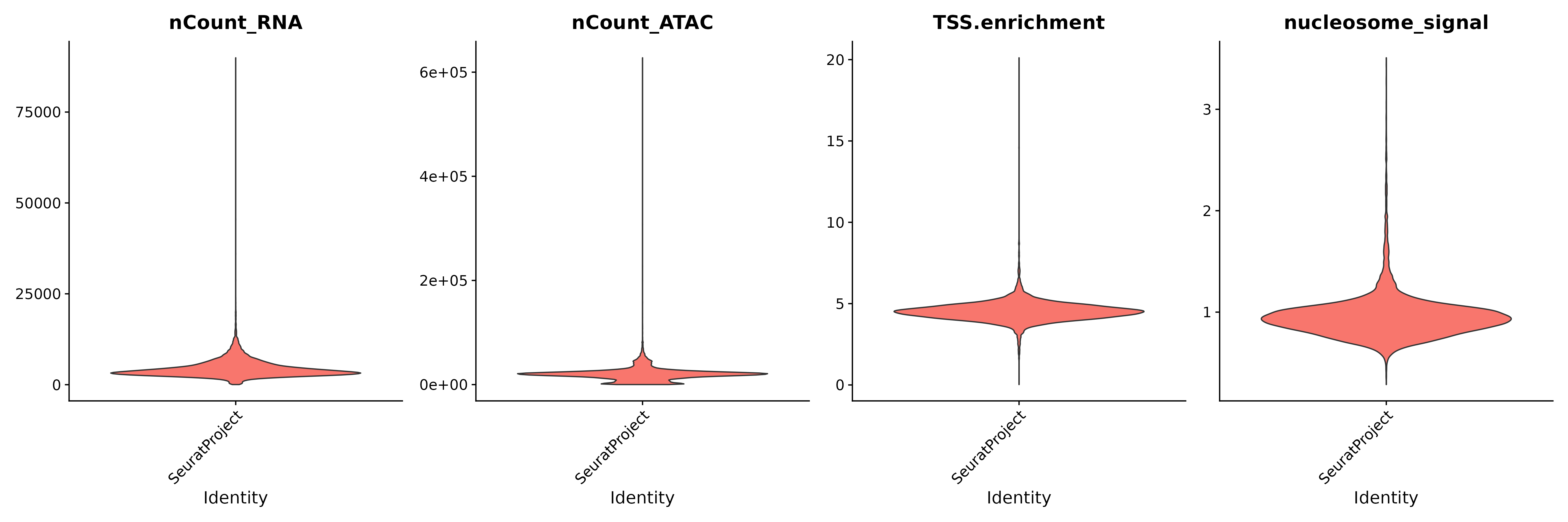
Calculate QC metrics (RNA counts, ATAC counts, nucleosome signal, TSS enrichment) and filter low-quality cells using defined thresholds.
# Set default assay to ATAC for ATAC-seq quality metrics calculation
DefaultAssay(pbmc) <- "ATAC"

# Calculate nucleosome signal score, which reflects nucleosome positioning
pbmc <- NucleosomeSignal(pbmc)

# Calculate Transcription Start Site (TSS) enrichment score for each cell, a metric for ATAC-seq data quality
pbmc <- TSSEnrichment(pbmc)

# Plot violin plots for QC metrics:
# - RNA counts per cell (nCount_RNA)
# - ATAC counts per cell (nCount_ATAC)
# - TSS enrichment score (TSS.enrichment)
# - Nucleosome signal score (nucleosome_signal)
VlnPlot(
  object = pbmc,
  features = c("nCount_RNA", "nCount_ATAC", "TSS.enrichment", "nucleosome_signal"),
  ncol = 4,
  pt.size = 0
)
# Filter out low-quality cells based on multiple QC thresholds
pbmc <- subset(
  x = pbmc,
  subset = nCount_ATAC < 100000 &
    nCount_RNA < 25000 &
    nCount_ATAC > 1000 &
    nCount_RNA > 1000 &
    nucleosome_signal < 2 &
    TSS.enrichment > 1
)

# Print summary of the filtered Seurat object
pbmc
## An object of class Seurat
## 144978 features across 11331 samples within 2 assays
## Active assay: ATAC (108377 features, 0 variable features)
## 2 layers present: counts, data
## 1 other assay present: RNAPeak calling and quantification
Call peaks, filter, count fragments per peak, and add to Seurat object.
# Call peaks using MACS2 from the fragments in the Seurat object
peaks <- CallPeaks(pbmc)

# Remove peaks on nonstandard chromosomes and in genomic blacklist regions
peaks <- keepStandardChromosomes(peaks, pruning.mode = "coarse")
peaks <- subsetByOverlaps(x = peaks, ranges = blacklist_hg38_unified, invert = TRUE)

# Quantify counts of fragments overlapping each peak for each cell, creating a peak-by-cell count matrix
macs2_counts <- FeatureMatrix(
  fragments = Fragments(pbmc),
  features = peaks,
  cells = colnames(pbmc)
)
## Extracting reads overlapping genomic regions
# Create a new chromatin assay based on MACS2-called peaks and add it to the Seurat object
pbmc[["peaks"]] <- CreateChromatinAssay(
  counts = macs2_counts,
  fragments = fragpath,
  annotation = annotation
)
## Computing hash
# Print summary of the updated Seurat object
pbmc
## An object of class Seurat
## 276342 features across 11331 samples within 3 assays
## Active assay: ATAC (108377 features, 0 variable features)
## 2 layers present: counts, data
## 2 other assays present: RNA, peaksRNA analysis
Normalize RNA data with SCTransform and perform PCA for dimensionality reduction.
# Set the default assay to "RNA" for RNA-based analysis
DefaultAssay(pbmc) <- "RNA"

# Perform normalization and variance stabilization using SCTransform
# This replaces traditional log-normalization and identifies variable features
pbmc <- SCTransform(pbmc)

# Run Principal Component Analysis (PCA) on the normalized data
# PCA reduces dimensionality while preserving major sources of variation
pbmc <- RunPCA(pbmc)
ATAC analysis
Identify highly accessible peaks and perform dimensionality reduction using TF-IDF and SVD (LSI).
# Set the default assay to "peaks" (i.e., the MACS2-called peak matrix)
DefaultAssay(pbmc) <- "peaks"

# Identify top features (peaks) based on accessibility; only keep peaks present in at least 5 cells
pbmc <- FindTopFeatures(pbmc, min.cutoff = 5)

# Perform Term Frequency-Inverse Document Frequency (TF-IDF) normalization
pbmc <- RunTFIDF(pbmc)

# Perform dimensionality reduction using Singular Value Decomposition (SVD), also referred to as Latent Semantic Indexing (LSI) in this context
pbmc <- RunSVD(pbmc)
Cell type annotation and integration analysis
We use an annotated PBMC reference dataset from Hao et al. (2020) to perform cell type annotation and integration. The reference dataset is publicly available at: https://atlas.fredhutch.org/data/nygc/multimodal/pbmc_multimodal.h5seurat.
# Load necessary library for working with Seurat h5Seurat format
library(SeuratDisk)

# Load multimodal PBMC reference dataset (processed with spca and SCT)
reference <- LoadH5Seurat("pbmc_multimodal.h5seurat", assays = list("SCT" = "counts"), reductions = "spca")

# Ensure the reference object is compatible with current Seurat version
reference <- UpdateSeuratObject(reference)

# Set the default assay for the query object to SCT (if applicable)
DefaultAssay(pbmc) <- "SCT"

# Identify anchors between the reference and the query using spca
transfer_anchors <- FindTransferAnchors(
  reference = reference,
  query = pbmc,
  normalization.method = "SCT",
  reference.reduction = "spca",
  recompute.residuals = FALSE,
  dims = 1:50
)

# Transfer cell type annotations from reference to query based on anchors
predictions <- TransferData(
  anchorset = transfer_anchors,
  refdata = reference$celltype.l1,
  weight.reduction = pbmc[["pca"]],
  dims = 1:50
)

# Store the predicted cell types in the metadata of the query object
pbmc <- AddMetaData(
  object = pbmc,
  metadata = predictions
)

# Set cell identities to the predicted labels
Idents(pbmc) <- "predicted.id"

# Set the display order of cell types
levels(pbmc) <- c("CD4 T", "CD8 T", "Mono", "NK", "B", "DC", "other T", "other")
Using Seurat v4’s weighted nearest neighbor method, we integrate gene expression and chromatin accessibility into a joint neighbor graph and create a unified UMAP embedding combining RNA and ATAC data.
# Build a multimodal nearest-neighbor graph using PCA from RNA and LSI from ATAC
pbmc <- FindMultiModalNeighbors(
  object = pbmc,
  reduction.list = list("pca", "lsi"),
  dims.list = list(1:50, 2:40),
  modality.weight.name = "RNA.weight",
  verbose = TRUE
)

# Generate a joint UMAP embedding using the WNN graph
# The embedding combines information from both RNA and ATAC modalities
pbmc <- RunUMAP(
  object = pbmc,
  nn.name = "weighted.nn",
  assay = "RNA",
  verbose = TRUE
)

DimPlot(pbmc, label = TRUE, repel = TRUE, reduction = "umap") + NoLegend()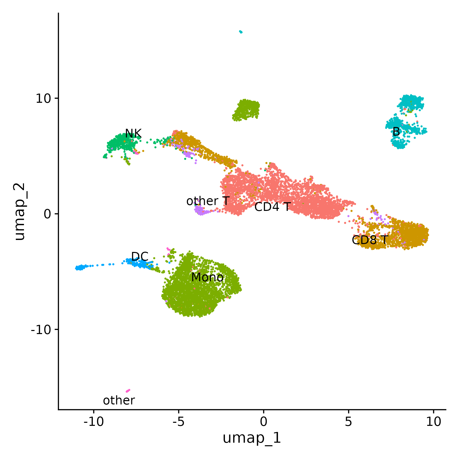
Infer enhancer–gene links
Preprocess data
When preprocessing data with SCEG-HiC, you can choose either aggregation or single-cell retention approach, and use either paired scATAC-seq/RNA-seq or scATAC-seq data alone. Here, we process paired scATAC-seq/RNA-seq data stored in a Seurat object using the aggregation approach. By default, the scATAC-seq counts are binarized to indicate the presence or absence of chromatin accessibility at each peak.
# Prepare input data for SCEG-HiC analysis
# This function processes paired scATAC-seq/RNA-seq data stored in a Seurat object
SCEGdata <- process_data(pbmc, max_overlap = 0.5)
## Generating aggregated data## Aggregating cluster CD4 T## Sample cells randomly.## There are 76 samples## Aggregating cluster CD8 T## Sample cells randomly.## There are 43 samples## Aggregating cluster Mono## Sample cells randomly.## There are 79 samples## Aggregating cluster NK## Sample cells randomly.## There are 12 samples## Aggregating cluster B## Sample cells randomly.## There are 20 samples## Aggregating cluster DC## Sample cells randomly.## There are 6 samples## Aggregating cluster other T## Sample cells randomly.## There are 6 samples## Aggregating cluster other## Skipping group other (not enough cells)Calculate weight
Calculating weights with SCEG-HiC can be time-consuming, especially as the number of selected genes increases. To facilitate this process, SCEG-HiC provides downloadable average Hi-C datasets for both human and mouse (detail here). In this case, we select the human average Hi-C data as prior information to calculate enhancer-gene links weights.
Select highly variable features
You can focus on the top 3000 highly variable genes identified by SCTransform normalization:
# Extract highly variable genes
gene <- pbmc@assays[["SCT"]]@var.features

# Calculate Hi-C weights for these genes using human average Hi-C data
weight <- calculateHiCWeights(SCEGdata, species = "Homo sapiens", genome = "hg38", focus_gene = gene, averHicPath = "/mnt/netshare2/liangxuan/data/human_contact/AvgHiC")
As an example, we calculate Hi-C weights focusing on PDK1, a key regulator of T cell development and activation.
# Alternatively, calculate Hi-C weights for PDK1
weight <- calculateHiCWeights(SCEGdata, species = "Homo sapiens", genome = "hg38", focus_gene = "PDK1", averHicPath = "/mnt/netshare2/liangxuan/data/human_contact/AvgHiC")
## Processing chromosome chr2...## Found 1 TSS loci on chr2.## Calculating Hi-C weights for gene PDK1...## Finished calculating Hi-C weights for all genes.Run model
SCEG-HiC employs the wglasso method to infer enhancer-gene links by integrating processed single-cell multi-omics data and normalized bulk average Hi-C contact matrices. The bulk Hi-C matrix is normalized using rank score to improve accuracy. In this example, we run the model focusing on genes PDK1 to identify their putative enhancer links.
# Example: Run the model focused on PDK1
results_SCEGHiC <- Run_SCEG_HiC(SCEGdata, weight, focus_gene = "PDK1")
## Total predicted genes: 1## Running model for gene: PDK1## [1] "The optimal penalty parameter (rho) selected by BIC is: 0.21"Visualize enhancer–gene links
Arc plot visualization of enhancer-gene links
Arc plot visualizes the predicted links between enhancers and target genes as arcs connecting genomic regions, highlighting spatial chromatin interactions inferred by SCEG-HiC.
Arc plot visualization of enhancer-gene links for PDK1.
# Download and prepare gene annotation data
# wget https://hgdownload2.soe.ucsc.edu/goldenPath/hg38/bigZips/genes/hg38.refGene.gtf.gz
temp <- "hg38.refGene.gtf.gz"
gene_anno <- rtracklayer::readGFF(temp)

# Rename some columns to match requirements
gene_anno$chromosome <- gene_anno$seqid
gene_anno$gene <- gene_anno$gene_id
gene_anno$transcript <- gene_anno$transcript_id
gene_anno$symbol <- gene_anno$gene_name

# Arc plot visualization of enhancer-gene links for PDK1
connections_Plot(results_SCEGHiC, species = "Homo sapiens", genome = "hg38", focus_gene = "PDK1", cutoff = 0.01, gene_anno = gene_anno)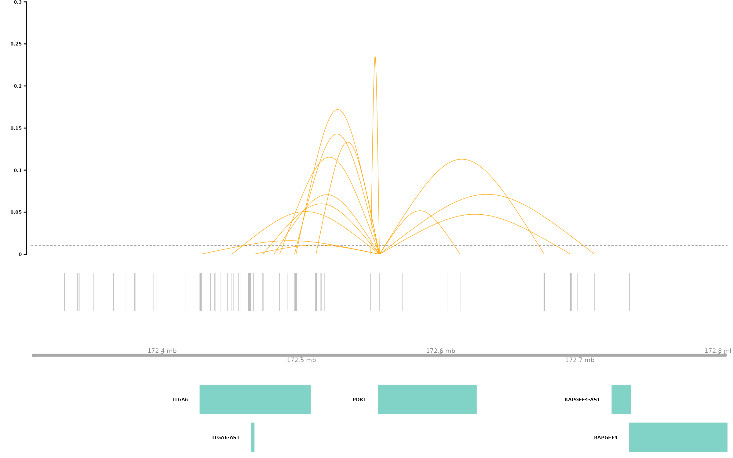
Coverage plot visualization of enhancer-gene links with Hi-C (or eQTL) validation
Coverage Plot visualizes chromatin accessibility around a target gene, including Hi-C interactions, scATAC-seq signals, aggregated ATAC-RNA correlations, eQTL SNPs, and enhancer–gene links predicted by SCEG-HiC. This facilitates intuitive comparison of regulatory interactions across multiple data layers.
Here, the ground truth for CD4+ T cells is obtained from the ENCODE database, and the correlation is calculated as the Pearson correlation coefficient between each gene and its candidate enhancers. The detailed code for this analysis is publicly available at the GitHub repository.
Coverage plot and visualize the links of PDK1.
# Load the truth of CD4+ T data
truth_CD4 <- readRDS("truth_CD4.rds")

## Load correlation data
correlation <- readRDS("correlation_CD4.rds")

# Coverage plot and visualize the links of PDK1
coverPlot(pbmc, focus_gene = "PDK1", species = "Homo sapiens", genome = "hg38", assay = "peaks", HIC_Result = truth_CD4, SCEG_HiC_Result = results_SCEGHiC, SCEG_HiC_cutoff = 0.01, correlation = correlation, cells = c("CD4 T", "CD8 T"))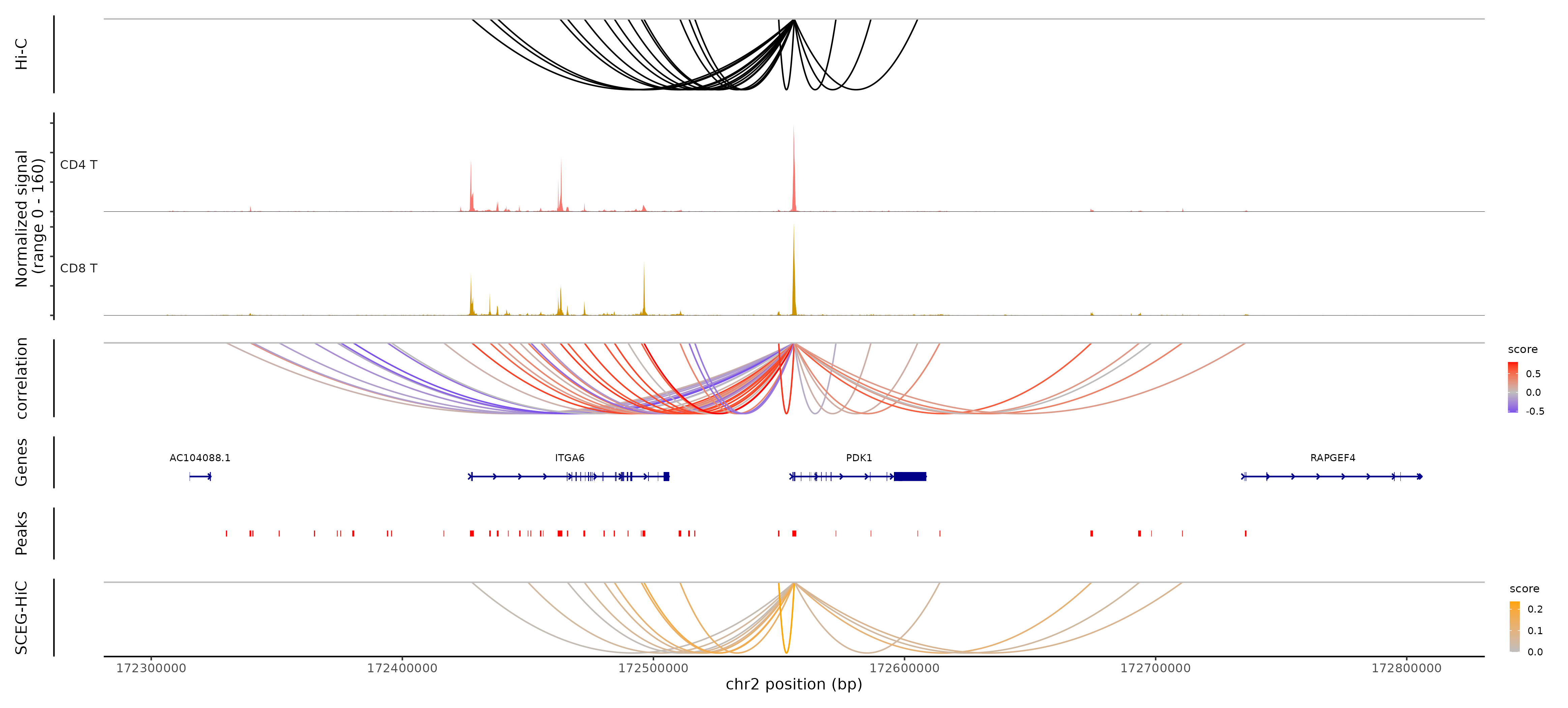
Session Info
## R version 4.4.2 (2024-10-31)
## Platform: x86_64-conda-linux-gnu
## Running under: Rocky Linux 9.6 (Blue Onyx)
##
## Matrix products: default
## BLAS/LAPACK: /home/liangxuan/conda/envs/test/lib/libopenblasp-r0.3.28.so;  LAPACK version 3.12.0
##
## locale:
##  [1] LC_CTYPE=en_US.UTF-8       LC_NUMERIC=C
##  [3] LC_TIME=en_US.UTF-8        LC_COLLATE=en_US.UTF-8
##  [5] LC_MONETARY=en_US.UTF-8    LC_MESSAGES=en_US.UTF-8
##  [7] LC_PAPER=en_US.UTF-8       LC_NAME=C
##  [9] LC_ADDRESS=C               LC_TELEPHONE=C
## [11] LC_MEASUREMENT=en_US.UTF-8 LC_IDENTIFICATION=C
##
## time zone: Asia/Shanghai
## tzcode source: system (glibc)
##
## attached base packages:
## [1] stats4    stats     graphics  grDevices datasets  utils     methods
## [8] base
##
## other attached packages:
##  [1] SeuratDisk_0.0.0.9021             hdf5r_1.3.12
##  [3] ggplot2_3.5.1                     BSgenome.Hsapiens.UCSC.hg38_1.4.5
##  [5] BSgenome_1.74.0                   rtracklayer_1.66.0
##  [7] BiocIO_1.16.0                     Biostrings_2.74.1
##  [9] XVector_0.46.0                    EnsDb.Hsapiens.v86_2.99.0
## [11] ensembldb_2.30.0                  AnnotationFilter_1.30.0
## [13] GenomicFeatures_1.58.0            AnnotationDbi_1.68.0
## [15] Biobase_2.66.0                    GenomicRanges_1.58.0
## [17] GenomeInfoDb_1.42.1               IRanges_2.40.1
## [19] S4Vectors_0.44.0                  BiocGenerics_0.52.0
## [21] Seurat_5.2.0                      SeuratObject_5.0.2
## [23] sp_2.1-4                          Signac_1.14.9001
## [25] SCEGHiC_1.0.1
##
## loaded via a namespace (and not attached):
##   [1] fs_1.6.5                    ProtGenerics_1.38.0
##   [3] matrixStats_1.5.0           spatstat.sparse_3.1-0
##   [5] bitops_1.0-9                httr_1.4.7
##   [7] RColorBrewer_1.1-3          tools_4.4.2
##   [9] sctransform_0.4.1           backports_1.5.0
##  [11] R6_2.5.1                    uwot_0.2.2
##  [13] lazyeval_0.2.2              Gviz_1.50.0
##  [15] cicero_1.3.9                withr_3.0.2
##  [17] prettyunits_1.2.0           gridExtra_2.3
##  [19] progressr_0.15.1            cli_3.6.3
##  [21] textshaping_1.0.1           spatstat.explore_3.3-4
##  [23] fastDummies_1.7.4           labeling_0.4.3
##  [25] slam_0.1-55                 sass_0.4.9
##  [27] spatstat.data_3.1-4         ggridges_0.5.6
##  [29] pbapply_1.7-2               pkgdown_2.1.1
##  [31] Rsamtools_2.22.0            systemfonts_1.1.0
##  [33] foreign_0.8-88              R.utils_2.12.3
##  [35] dichromat_2.0-0.1           parallelly_1.41.0
##  [37] VGAM_1.1-12                 rstudioapi_0.17.1
##  [39] RSQLite_2.3.9               FNN_1.1.4.1
##  [41] generics_0.1.3              ica_1.0-3
##  [43] spatstat.random_3.3-2       dplyr_1.1.4
##  [45] Matrix_1.6-5                interp_1.1-6
##  [47] ggbeeswarm_0.7.2            abind_1.4-8
##  [49] R.methodsS3_1.8.2           lifecycle_1.0.4
##  [51] yaml_2.3.10                 SummarizedExperiment_1.36.0
##  [53] SparseArray_1.6.0           BiocFileCache_2.14.0
##  [55] Rtsne_0.17                  grid_4.4.2
##  [57] blob_1.2.4                  promises_1.3.2
##  [59] crayon_1.5.3                miniUI_0.1.1.1
##  [61] lattice_0.22-6              cowplot_1.1.3
##  [63] KEGGREST_1.46.0             pillar_1.10.1
##  [65] knitr_1.49                  boot_1.3-31
##  [67] rjson_0.2.23                future.apply_1.11.3
##  [69] codetools_0.2-20            fastmatch_1.1-6
##  [71] glue_1.8.0                  spatstat.univar_3.1-1
##  [73] data.table_1.16.4           Rdpack_2.6.2
##  [75] vctrs_0.6.5                 png_0.1-8
##  [77] spam_2.11-0                 gtable_0.3.6
##  [79] assertthat_0.2.1            cachem_1.1.0
##  [81] xfun_0.50                   rbibutils_2.3
##  [83] S4Arrays_1.6.0              mime_0.12
##  [85] reformulas_0.4.0            survival_3.8-3
##  [87] SingleCellExperiment_1.28.1 RcppRoll_0.3.1
##  [89] fitdistrplus_1.2-2          ROCR_1.0-11
##  [91] nlme_3.1-166                bit64_4.5.2
##  [93] progress_1.2.3              filelock_1.0.3
##  [95] RcppAnnoy_0.0.22            bslib_0.8.0
##  [97] irlba_2.3.5.1               vipor_0.4.7
##  [99] KernSmooth_2.23-26          rpart_4.1.24
## [101] colorspace_2.1-1            DBI_1.2.3
## [103] Hmisc_5.2-2                 nnet_7.3-20
## [105] ggrastr_1.0.2               tidyselect_1.2.1
## [107] bit_4.5.0.1                 compiler_4.4.2
## [109] curl_6.0.1                  httr2_1.0.7
## [111] htmlTable_2.4.3             xml2_1.5.0
## [113] desc_1.4.3                  DelayedArray_0.32.0
## [115] plotly_4.10.4               checkmate_2.3.2
## [117] scales_1.4.0                lmtest_0.9-40
## [119] rappdirs_0.3.3              stringr_1.5.1
## [121] digest_0.6.37               goftest_1.2-3
## [123] minqa_1.2.8                 spatstat.utils_3.1-2
## [125] reader_1.0.6                rmarkdown_2.29
## [127] htmltools_0.5.8.1           pkgconfig_2.0.3
## [129] jpeg_0.1-10                 base64enc_0.1-3
## [131] lme4_1.1-36                 MatrixGenerics_1.18.1
## [133] dbplyr_2.5.0                fastmap_1.2.0
## [135] rlang_1.1.4                 htmlwidgets_1.6.4
## [137] UCSC.utils_1.2.0            shiny_1.10.0
## [139] farver_2.1.2                jquerylib_0.1.4
## [141] zoo_1.8-12                  jsonlite_1.8.9
## [143] BiocParallel_1.40.0         R.oo_1.27.0
## [145] VariantAnnotation_1.52.0    RCurl_1.98-1.16
## [147] magrittr_2.0.3              Formula_1.2-5
## [149] GenomeInfoDbData_1.2.13     dotCall64_1.2
## [151] patchwork_1.3.0             Rcpp_1.0.14
## [153] reticulate_1.40.0           stringi_1.8.7
## [155] zlibbioc_1.52.0             MASS_7.3-64
## [157] plyr_1.8.9                  parallel_4.4.2
## [159] listenv_0.9.1               ggrepel_0.9.6
## [161] deldir_2.0-4                splines_4.4.2
## [163] tensor_1.5                  hms_1.1.3
## [165] igraph_2.0.3                spatstat.geom_3.3-4
## [167] RcppHNSW_0.6.0              reshape2_1.4.4
## [169] biomaRt_2.62.0              XML_3.99-0.17
## [171] evaluate_1.0.3              latticeExtra_0.6-30
## [173] biovizBase_1.54.0           renv_1.0.11
## [175] BiocManager_1.30.27         NCmisc_1.2.0
## [177] nloptr_2.1.1                tweenr_2.0.3
## [179] httpuv_1.6.15               RANN_2.6.2
## [181] tidyr_1.3.1                 purrr_1.0.2
## [183] polyclip_1.10-7             future_1.34.0
## [185] scattermore_1.2             ggforce_0.4.2
## [187] monocle3_1.3.7              xtable_1.8-4
## [189] restfulr_0.0.15             RSpectra_0.16-2
## [191] later_1.4.1                 glasso_1.11
## [193] viridisLite_0.4.2           ragg_1.3.3
## [195] tibble_3.2.1                beeswarm_0.4.0
## [197] memoise_2.0.1               GenomicAlignments_1.42.0
## [199] cluster_2.1.8               globals_0.16.3