
Overview
SCEG-HiC predicts enhancer–gene links by integrating multi-omics single-cell data (either paired scATAC-seq/RNA-seq or scATAC-seq alone) with three-dimensional chromatin conformation information derived from bulk average Hi-C data. It employs the weighted graphical lasso (wglasso) model to incorporate average bulk Hi-C data, effectively regularizing the correlation matrix with the prior Hi-C contact matrix as a penalty term.
Installation
Required software
SCEG-HiC runs in the R statistical computing environment. It requires R version 4.1.0 or higher, Bioconductor version 3.14 or higher, and Seurat 4.0 or higher to access the latest features.
To install Bioconductor, open an R session and run:
if (!requireNamespace("BiocManager", quietly = TRUE))
    install.packages("BiocManager")
BiocManager::install(version = "3.14")
Next, install a few Bioconductor packages that are not installed automatically:
BiocManager::install(c(
  'BiocGenerics', 'DelayedArray', 'DelayedMatrixStats',
  'limma', 'lme4', 'S4Vectors', 'SingleCellExperiment',
  'SummarizedExperiment', 'batchelor', 'HDF5Array',
  'terra', 'ggrastr', 'Gviz', 'rtracklayer', 'GenomeInfoDb', 'GenomicRanges'
))
Installation of other dependencies
- Install the Signac pacakge:
devtools::install_github("timoast/signac", ref = "develop"). If you encounter any issues, please check the Signac documentation. - Install the Cicero package:
devtools::install_github("cole-trapnell-lab/cicero-release", ref = "monocle3"). If you encounter any issues, please check the Cicero installation guide.
Now, you can install the development version of SCEG-HiC from GitHub with:
# If you haven't installed devtools yet, uncomment and run:
# install.packages("devtools")

# Install the development version of SCEG-HiC from GitHub
devtools::install_github("wuwei77lx/SCEGHiC")
If you prefer the stable release version from CRAN, run:
# Install the released version from CRAN
install.packages("SCEGHiC")Quickstart
This basic example demonstrates how to analyze paired scATAC-seq/RNA-seq data using SCEG-HiC:
library(SCEGHiC)
library(Signac)

# Load example multi-omics dataset
data(multiomic_small)

# Preprocess the data (aggregation)
SCEGdata <- process_data(multiomic_small, k_neigh = 5, max_overlap = 0.5)
#> Generating aggregated data
#> Aggregating cluster 0
#> Sample cells randomly.
#> There are 11 samples
#> Aggregating cluster 1
#> Sample cells randomly.
#> There are 11 samples

# Define genes of interest
gene <- c("TRABD2A", "GNLY", "MFSD6", "CTLA4", "LCLAT1", "NCK2", "GALM", "TMSB10", "ID2", "CXCR4")

# Get path to example average Hi-C data
fpath <- system.file("extdata", package = "SCEGHiC")

# Calculate Hi-C based weights for enhancer-gene pairs
weight <- calculateHiCWeights(SCEGdata, species = "Homo sapiens", genome = "hg38", focus_gene = gene, averHicPath = fpath)
#> Processing chromosome chr2...
#> Found 10 TSS loci on chr2.
#> Calculating Hi-C weights for gene TRABD2A...
#> Calculating Hi-C weights for gene GNLY...
#> Calculating Hi-C weights for gene MFSD6...
#> Calculating Hi-C weights for gene CXCR4...
#> Calculating Hi-C weights for gene CTLA4...
#> Calculating Hi-C weights for gene LCLAT1...
#> Calculating Hi-C weights for gene NCK2...
#> Calculating Hi-C weights for gene ID2...
#> Calculating Hi-C weights for gene GALM...
#> Calculating Hi-C weights for gene TMSB10...
#> Finished calculating Hi-C weights for all genes.

# Run the SCEG-HiC model
results_SCEGHiC <- Run_SCEG_HiC(SCEGdata, weight, focus_gene = gene)
#> Total predicted genes: 10
#> Running model for gene: TRABD2A
#> [1] "The optimal penalty parameter (rho) selected by BIC is: 0.43"
#> Running model for gene: GNLY
#> [1] "The optimal penalty parameter (rho) selected by BIC is: 0.19"
#> Running model for gene: MFSD6
#> [1] "The optimal penalty parameter (rho) selected by BIC is: 0.22"
#> Running model for gene: CXCR4
#> [1] "The optimal penalty parameter (rho) selected by BIC is: 0.14"
#> Running model for gene: CTLA4
#> [1] "The optimal penalty parameter (rho) selected by BIC is: 0.17"
#> Running model for gene: LCLAT1
#> [1] "The optimal penalty parameter (rho) selected by BIC is: 0.41"
#> Running model for gene: NCK2
#> [1] "The optimal penalty parameter (rho) selected by BIC is: 0.25"
#> Running model for gene: ID2
#> [1] "The optimal penalty parameter (rho) selected by BIC is: 0.13"
#> Running model for gene: GALM
#> [1] "The optimal penalty parameter (rho) selected by BIC is: 0.11"
#> Running model for gene: TMSB10
#> [1] "The optimal penalty parameter (rho) selected by BIC is: 0.44"

# Arc plot visualization predicted enhancer-gene links for CTLA4
connections_Plot(results_SCEGHiC, species = "Homo sapiens", genome = "hg38", focus_gene = "CTLA4", cutoff = 0.01, gene_anno = NULL)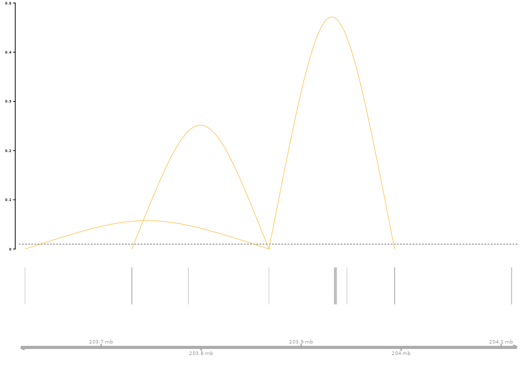
# Load fragment data for coverage plotting
frag_path <- system.file("extdata", "multiomic_small_atac_fragments.tsv.gz", package = "SCEGHiC")
frags <- CreateFragmentObject(path = frag_path, cells = colnames(multiomic_small))
#> Computing hash
Fragments(multiomic_small) <- frags

# Coverage plot and visualize the links of CTLA4
coverPlot(multiomic_small, focus_gene = "CTLA4", species = "Homo sapiens", genome = "hg38",
          assay = "peaks", SCEG_HiC_Result = results_SCEGHiC, SCEG_HiC_cutoff = 0.01)
#> Warning in .merge_two_Seqinfo_objects(x, y): The 2 combined objects have no sequence levels in common. (Use
#>   suppressWarnings() to suppress this warning.)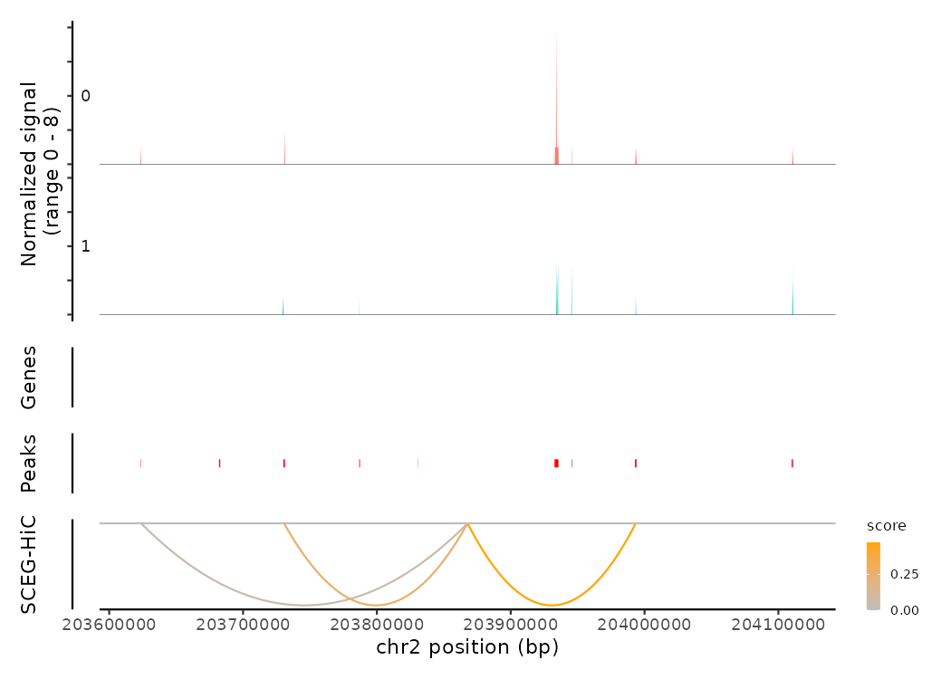
Session Info
sessionInfo()
#> R version 4.4.2 (2024-10-31)
#> Platform: x86_64-conda-linux-gnu
#> Running under: Rocky Linux 9.6 (Blue Onyx)
#>
#> Matrix products: default
#> BLAS/LAPACK: /home/liangxuan/conda/envs/test/lib/libopenblasp-r0.3.28.so;  LAPACK version 3.12.0
#>
#> locale:
#>  [1] LC_CTYPE=en_US.UTF-8       LC_NUMERIC=C
#>  [3] LC_TIME=en_US.UTF-8        LC_COLLATE=en_US.UTF-8
#>  [5] LC_MONETARY=en_US.UTF-8    LC_MESSAGES=en_US.UTF-8
#>  [7] LC_PAPER=en_US.UTF-8       LC_NAME=C
#>  [9] LC_ADDRESS=C               LC_TELEPHONE=C
#> [11] LC_MEASUREMENT=en_US.UTF-8 LC_IDENTIFICATION=C
#>
#> time zone: Asia/Shanghai
#> tzcode source: system (glibc)
#>
#> attached base packages:
#> [1] stats     graphics  grDevices utils     datasets  methods   base
#>
#> other attached packages:
#> [1] Signac_1.14.9001 SCEGHiC_1.0.1
#>
#> loaded via a namespace (and not attached):
#>   [1] spatstat.sparse_3.1-0       fs_1.6.5
#>   [3] ProtGenerics_1.38.0         matrixStats_1.5.0
#>   [5] bitops_1.0-9                devtools_2.4.5
#>   [7] httr_1.4.7                  RColorBrewer_1.1-3
#>   [9] sctransform_0.4.1           profvis_0.4.0
#>  [11] tools_4.4.2                 backports_1.5.0
#>  [13] R6_2.5.1                    uwot_0.2.2
#>  [15] lazyeval_0.2.2              Gviz_1.50.0
#>  [17] cicero_1.3.9                urlchecker_1.0.1
#>  [19] withr_3.0.2                 sp_2.1-4
#>  [21] prettyunits_1.2.0           gridExtra_2.3
#>  [23] progressr_0.15.1            textshaping_1.0.1
#>  [25] cli_3.6.3                   Biobase_2.66.0
#>  [27] spatstat.explore_3.3-4      fastDummies_1.7.4
#>  [29] labeling_0.4.3              slam_0.1-55
#>  [31] Seurat_5.2.0                spatstat.data_3.1-4
#>  [33] ggridges_0.5.6              pbapply_1.7-2
#>  [35] pkgdown_2.1.1               systemfonts_1.1.0
#>  [37] commonmark_1.9.2            Rsamtools_2.22.0
#>  [39] foreign_0.8-88              R.utils_2.12.3
#>  [41] dichromat_2.0-0.1           parallelly_1.41.0
#>  [43] sessioninfo_1.2.2           BSgenome_1.74.0
#>  [45] VGAM_1.1-12                 rstudioapi_0.17.1
#>  [47] RSQLite_2.3.9               FNN_1.1.4.1
#>  [49] generics_0.1.3              BiocIO_1.16.0
#>  [51] spatstat.random_3.3-2       ica_1.0-3
#>  [53] dplyr_1.1.4                 Matrix_1.6-5
#>  [55] interp_1.1-6                S4Vectors_0.44.0
#>  [57] abind_1.4-8                 R.methodsS3_1.8.2
#>  [59] lifecycle_1.0.4             yaml_2.3.10
#>  [61] SummarizedExperiment_1.36.0 SparseArray_1.6.0
#>  [63] BiocFileCache_2.14.0        Rtsne_0.17
#>  [65] grid_4.4.2                  blob_1.2.4
#>  [67] promises_1.3.2              crayon_1.5.3
#>  [69] miniUI_0.1.1.1              lattice_0.22-6
#>  [71] cowplot_1.1.3               GenomicFeatures_1.58.0
#>  [73] KEGGREST_1.46.0             pillar_1.10.1
#>  [75] knitr_1.49                  GenomicRanges_1.58.0
#>  [77] rjson_0.2.23                boot_1.3-31
#>  [79] future.apply_1.11.3         codetools_0.2-20
#>  [81] fastmatch_1.1-6             glue_1.8.0
#>  [83] spatstat.univar_3.1-1       data.table_1.16.4
#>  [85] remotes_2.5.0               vctrs_0.6.5
#>  [87] png_0.1-8                   spam_2.11-0
#>  [89] Rdpack_2.6.2                gtable_0.3.6
#>  [91] assertthat_0.2.1            cachem_1.1.0
#>  [93] xfun_0.50                   rbibutils_2.3
#>  [95] S4Arrays_1.6.0              mime_0.12
#>  [97] reformulas_0.4.0            survival_3.8-3
#>  [99] SingleCellExperiment_1.28.1 RcppRoll_0.3.1
#> [101] ellipsis_0.3.2              fitdistrplus_1.2-2
#> [103] ROCR_1.0-11                 nlme_3.1-166
#> [105] usethis_3.1.0               bit64_4.5.2
#> [107] progress_1.2.3              filelock_1.0.3
#> [109] RcppAnnoy_0.0.22            GenomeInfoDb_1.42.1
#> [111] rprojroot_2.0.4             irlba_2.3.5.1
#> [113] KernSmooth_2.23-26          rpart_4.1.24
#> [115] colorspace_2.1-1            BiocGenerics_0.52.0
#> [117] DBI_1.2.3                   Hmisc_5.2-2
#> [119] nnet_7.3-20                 processx_3.8.5
#> [121] tidyselect_1.2.1            bit_4.5.0.1
#> [123] compiler_4.4.2              curl_6.0.1
#> [125] httr2_1.0.7                 htmlTable_2.4.3
#> [127] xml2_1.5.0                  plotly_4.10.4
#> [129] desc_1.4.3                  DelayedArray_0.32.0
#> [131] rtracklayer_1.66.0          checkmate_2.3.2
#> [133] scales_1.4.0                lmtest_0.9-40
#> [135] callr_3.7.6                 rappdirs_0.3.3
#> [137] goftest_1.2-3               stringr_1.5.1
#> [139] digest_0.6.37               spatstat.utils_3.1-2
#> [141] minqa_1.2.8                 reader_1.0.6
#> [143] rmarkdown_2.29              XVector_0.46.0
#> [145] htmltools_0.5.8.1           pkgconfig_2.0.3
#> [147] jpeg_0.1-10                 base64enc_0.1-3
#> [149] lme4_1.1-36                 MatrixGenerics_1.18.1
#> [151] dbplyr_2.5.0                fastmap_1.2.0
#> [153] ensembldb_2.30.0            rlang_1.1.4
#> [155] htmlwidgets_1.6.4           UCSC.utils_1.2.0
#> [157] shiny_1.10.0                farver_2.1.2
#> [159] zoo_1.8-12                  jsonlite_1.8.9
#> [161] BiocParallel_1.40.0         R.oo_1.27.0
#> [163] VariantAnnotation_1.52.0    RCurl_1.98-1.16
#> [165] magrittr_2.0.3              Formula_1.2-5
#> [167] GenomeInfoDbData_1.2.13     dotCall64_1.2
#> [169] patchwork_1.3.0             Rcpp_1.0.14
#> [171] reticulate_1.40.0           stringi_1.8.7
#> [173] zlibbioc_1.52.0             MASS_7.3-64
#> [175] plyr_1.8.9                  pkgbuild_1.4.5
#> [177] ggrepel_0.9.6               parallel_4.4.2
#> [179] listenv_0.9.1               deldir_2.0-4
#> [181] Biostrings_2.74.1           splines_4.4.2
#> [183] tensor_1.5                  hms_1.1.3
#> [185] ps_1.8.1                    igraph_2.0.3
#> [187] spatstat.geom_3.3-4         RcppHNSW_0.6.0
#> [189] reshape2_1.4.4              biomaRt_2.62.0
#> [191] stats4_4.4.2                pkgload_1.4.0
#> [193] XML_3.99-0.17               evaluate_1.0.3
#> [195] SeuratObject_5.0.2          latticeExtra_0.6-30
#> [197] biovizBase_1.54.0           NCmisc_1.2.0
#> [199] nloptr_2.1.1                tweenr_2.0.3
#> [201] httpuv_1.6.15               RANN_2.6.2
#> [203] tidyr_1.3.1                 purrr_1.0.2
#> [205] polyclip_1.10-7             scattermore_1.2
#> [207] future_1.34.0               ggplot2_3.5.1
#> [209] ggforce_0.4.2               xtable_1.8-4
#> [211] monocle3_1.3.7              restfulr_0.0.15
#> [213] AnnotationFilter_1.30.0     RSpectra_0.16-2
#> [215] roxygen2_7.3.3              later_1.4.1
#> [217] ragg_1.3.3                  viridisLite_0.4.2
#> [219] glasso_1.11                 tibble_3.2.1
#> [221] memoise_2.0.1               AnnotationDbi_1.68.0
#> [223] GenomicAlignments_1.42.0    IRanges_2.40.1
#> [225] cluster_2.1.8               globals_0.16.3
See the documentation website for more information!
The bulk average Hi-C data
The human cell types used for averaging are based on 34 Hi-C datasets from the ENCODE project.
The mouse cell types used for averaging are: two embryonic stem cell types (mESC1, mESC2), CH12LX, CH12F3, fiber, epithelium, and B cells.
The bulk average Hi-C data can be generated using the Activity by Contact (ABC) model’s makeAverageHiC.py script.
Download Links for Average Hi-C Data
-
Human bulk average Hi-C (~54.1 GB)
Download from: ENCFF134PUN.bed.gz.
After downloading, extract the human bulk average Hi-C using the Activity by Contact (ABC) model’s extract_avg_hic.py script:
-
Mouse bulk average Hi-C (~13.9 GB)
Download from: 10.5281/zenodo.14849886.
For more details about bulk average Hi-C data, please visit: https://github.com/wuwei77lx/compare_model.
Example
In SCEG-HiC, you can choose either aggregation or single-cell retention approach:
Aggregation approach: Aggregates binarized scATAC-seq data across cell types using k-nearest neighbor smoothing to reduce data sparsity. This approach captures a broader spectrum of enhancer-gene links across cell types, with slightly reduced prediction accuracy.
Single-cell retention approach: Normalizes scATAC-seq data within individual cell types to individual cell signals. This method achieves higher precision and accuracy, albeit identifying fewer enhancer-gene links
Recommendation: To balance accuracy and coverage, we implemented both preprocessing strategies in SCEG-HiC, with aggregation designated as the default. The single-cell retention approach can be optionally used when higher precision within specific cell types is desired.
For more details and real data examples, please visit:
SCEG-HiC on paired scATAC-seq/RNA-seq data of PBMC (aggregation)
SCEG-HiC on paired scATAC-seq/RNA-seq data of mouse skin (aggregation)
SCEG-HiC on scATAC-seq data alone from human COVID-19 monocytes
Alternatively, when applying SCEG-HiC to a new tissue, the penalty strength can be adjusted using the alpha parameter (alpha * rho):
Increase alpha is suitable for tissues well represented in the datasets used to construct the bulk average Hi-C map, to allow greater reliance on prior Hi-C contact information.
Decrease alpha is preferable for more unique tissues or conditions, to reduce dependence on prior Hi-C contact information and emphasize single-cell data.
# Example: run SCEG-HiC with scaled penalty
results_SCEGHiC <- Run_SCEG_HiC(SCEGdata, weight, focus_gene = gene, alpha=1.5)
Notes:
alpha = 1uses the original penalty (default).alpha > 1strengthens the penalty.alpha < 1weakens the penalty.
Help
If you have any questions, comments, or suggestions, please contact Xuan Liang at liangxuan2022@sinh.ac.cn.